BML FPGA Design Tutorial Part-6ofN

Digital Logic Simulation at the RTL level using AMD/Xilinx Vivado Simulator and GTKWave.

2024.06.09 : I’m Kevin Hubbard, Electrical Engineer who has been designing digital logic circuits for 45 of my 55 years on this planet. 30 some years ago I got my BSEE degree and have been designing ASICs and FPGAs ever since. I’m giving back now in writing this “Getting started with FPGAs” series.

In Part-5 of this tutorial ( starts here ), I explained RTL simulations using the ModelSim simulator. In Part-6 I will explain doing the same, but using the simulator that is included with AMD/Xilinx Vivado tool available for download here. For the back-end viewing of waveform files, I will use the excellent GTKwave VCD viewer. Note, a lot of this information is also available in and older post from 2018 where I explained using my Sump2.py logic analyzer as a VCD viewer for Vivado’s simulator.

Step-1 is to create the top.v file to simulate.

[ top.v ]

timescale 1 ns/ 100 ps default_nettype none // Strictly enforce all nets to be declared

module top
(
  input wire clk,
  output wire [3:0] led
);// module top

  wire clk_100m_loc;
  wire clk_100m_tree;
  reg [3:0] my_cnt = 4'd0;
  wire pulse_1hz = 1;

  assign clk_100m_loc = clk; // infer IBUF
  assign clk_100m_tree = clk_100m_loc; // infer BUFG

always @ ( posedge clk_100m_tree ) begin
  if ( pulse_1hz == 1 ) begin
    my_cnt <= my_cnt[3:0] + 1;
  end
end
  assign led = my_cnt[3:0];

endmodule // top.v
`default_nettype wire // enable Verilog default for any 3rd party IP needing it

This Verilog RTL now needs to be compiled prior to simulation. The first file to create is a “project” file which points to one or more Verilog ( and/or VHDL ) design source files.

[ top.prj ]

verilog work "$XILINX_VIVADO/data/verilog/src/glbl.v"
verilog work "top.v"

Note the “glbl.v” file, it’s a necessary evil for running Verilog simulations on both ModelSim and VivadoSim. This 1st line tells the simulator to compile “glbl.v” from the Vivado install path.

Now that we have a project file, it’s time to create a compile script. This can be a UNIX shell script or a MS-DOS batch file – it makes no difference – just change the file extension from *.sh to *.bat if you are still stuck in a 1980’s MS-DOS world.

[ compile.sh ]

xvlog -prj top.prj

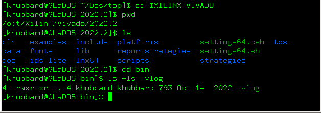
This script is rather boring. It’s telling the OS ( Linux, a real OS in my case ) to launch the command line executable “xvlog” in the Vivado install path and pass it the name ( and location ) of the project file to use. Below I hunted down the location of “xvlog” and it is tiny at only 793 bytes. It turns out that “xvlog” is just another shell script that calls another program – that’s actually a compiled binary. EDA tools can be like that and is one of the interesting evolutions of UNIX / Linux. It’s quite practical to have a single monolithic binary and have multiple shell scripts call it while they pretend to be different tools from the command line. Gets the job done. I’m not complaining.

Compiling the design is as easy as typing “source compile.sh”. If there are any syntax errors in “top.v”, they will be reported in STDOUT.

In this below example I deliberately typed a syntax error in “top.v”. The compiler spit out the error message both to STDOUT and the file “xvlog.log”. The latter is super handy when compiling hundreds of files at once as the number of errors may rapidly scroll off the STDOUT console screen.

So what did compiling “top.v” and “glbl.v” accomplish? We have to dig down into the subdirectory ./xsim.dir/work to see that it generated 3 new files.

The file “work.rlx” is actually a text file. It appears to be a table of contents for what is in the work directory including full hard paths to the source files. In a pinch a person could work backwards to figure out where a design was compiled from. The two *.sdb files “glbl.sdb” and “top.sdb” are purely binaries. I think of them as pseudo “Java Byte Code” representations of the compiled Verilog.

Now that “top.v” ( and “glbl.v” ) are compiled, it’s time to simulate them. We will create a “simulate.sh” command line script ( or “*.bat” ) that looks like this:

[ simulate.sh ]

xelab top glbl -prj top.prj -s snapshot -debug typical -initfile=$XILINX_VIVADO/data/xsim/ip/xsim_ip.ini -L work -L xpm -L unisims_ver -L unimacro_ver
xsim snapshot -tclbatch do_files/do.tcl

Wow – that’s certainly a lot to take in. Let’s digest it piece by piece.
The first line with “xelab” takes some explaining. With the “-s snapshot” option, it will generate a “snapshot.wdb” binary file that is a single simulation “executable” of the compiled Verilog ( of “top.v” and “glbl.v” ) as well as a long list of pre-compiled AMD/Xilinx library primitives that are all linked with the “-L” flag.
These primitives are for things like flip-flops, clock tree buffers, SERDES transceivers. What’s important to know is that any user generated IP for things like FIFOs will require these libraries for simulation. It’s a key advantage to using VivadoSim over other simulators as all of the primitives are already included and pre-compiled, ready to be simulated.

The second line with “xsim snapshot -tclbatch do_files/do.tcl” says to simulate the “snapshot.wdb” binary file and apply stimulus as specified in the “do.tcl” file. What’s in “do.tcl” ? A bunch of stuff. Note that “do_files” is just an optional subdirectory “./do_files/” where I chose to dump all my stimulus files in one place. I could have named the directory “./asparagus/” instead – or left everything flat at one directory level.

[ do.tcl ]

open_vcd
source do_files/wave.tcl
source do_files/force.tcl
close_vcd
quit

Line-by-line breakdown:
“open_vcd” : Instructs the simulator to create a new VCD file to store simulator results to.
“source do_files/wave.tcl” : Instructs the simulator to execute an external file.
“source do_files/force.tcl” : Instructs the simulator to execute another external file.
“close_vcd” : Instructs the simulator to close out the newly created VCD file.
“quit” : Instructs the simulator to stop and exit back to the OS command line.

[ wave.tcl ]

log_vcd [get_objects -r * ]
#log_vcd {clk_wr}
#log_vcd {/fifo_1024x36/clk_wr}

The “wave.tcl” file specifies which signals to put in the output VCD file. The 1st line ( that has no preceding comment ) says to capture ALL signals of the design. The next two commented lines show how to capture only certain signals at certain hierarchy instance levels.

[ force.tcl ]

#add_force reset 1
add_force clk {0 0ns} {1 5000ps} -repeat_every 10ns
run 50ns
#add_force reset 0
run 600ns

The “force.tcl” provides actually stimulus to the design. The “top.v” doesn’t have a reset input, but if it did, the commented out “add_force reset” lines show how to force an input pin to one state or another. The “add_force clk” line specifies a repeating 100 MHz ( 10 ns ) clock of 50/50 duty cycle. The “run” commands tell the simulator the length of time to simulate between force commands. If you have wide inputs, you can specify a non-binary radix, for example “add_force my_byte AA -radix hex”.

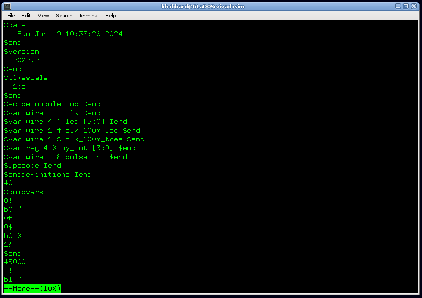
After running “simulate.sh”, the simulator will spit out “dump.vcd”. VCD files are clear text files containing Run Length Encoded binary representations of signals. They are not intended to be read by humans. That said, if you study them long enough, they are far easier to decipher than some Enigma encrypted proprietary binary file format.

Viewing “dump.vcd” using GTKWave is simply a matter of opening the file and selecting the signals to view. For this simple design I clicked on “top” which then displayed all of the signal names on the left bottom pane. I selected “clk” and “led[3:0]” and clicked “Append” which added those and only those two signals to the waveform display. The GTKWave GitHub site is here. The pre-compiled executables are available here. GTKWave is an excellent viewer that I can’t recommend enough. It’s true that Vivado has an internal waveform viewer. I’m not interested.

As a footnote, ModelSim will also happily display the output VCD file for you. You just need to convert from VCD to WLF format using the command line tool called (wait for it)…… “vcd2wlf” that is included with ModelSim.
“vcd2wlf dump.vcd dump.wlf”.

Why can’t you just launch vsim with a “-view dump.vcd” flag? That’s a very good question.

Using ModelSim to view VCD results from VivadoSim may seem silly, but I’ve actually used this path many times. Simulating hard or encrypted IP blocks from AMD/Xilinx can be a difficult using ModelSim and they often just work with VivadoSim. I’m not familiar with the VivadoSim GUI though. Running the simulation with VivadoSim and viewing the results with ModelSim is actually my preferred path. This isn’t implying that GTKWave isn’t great ( it is ) – I’m just used to using ModelSim. I have an install tutorial here.

That’s it for Part-6 of my little FPGA tutorial. In Part-7 I explain design hierarchy and how I use my open-source ChipVault IDE to easily manage hundreds of RTL design files.

EOF